Excel - Volatile Functions

I have a couple of questions about volatile functions in Excel.

General education question - According to multiple sources on the internet, =CELL() is a volatile function under certain circumstances/depending on what arguments are used. What are those circumstances/arguments?

Real life application - =OFFSET() is a volatile function. What is a good alternative? I have a spreadsheet that looks for a value from 12 months ago (i.e., 11 columns to the left). I also have some equations that sum up the last 12 months of data (i.e. & e.g., sum one row above the current cell and the 11 columns to the left of that). Because of the way I update the thing on a monthly basis, I was using OFFSET because direct references got messed up in the update.

If the performance of my spreadsheet is adequate (i.e., I only have a few offset functions & it’s not a huge calculation monster) do I need to worry about removing OFFSET?

My one use of CELL is =CELL(“filename”), which is volatile.

Looking at the documentation for the function: https://support.microsoft.com/en-us/office/cell-function-51bd39a5-f338-4dbe-a33f-955d67c2b2cf

It doesn’t say which are volatile and which aren’t.

If you have the dates on the columns/rows to label them, you might be able to use SUMIFS to get what you want.

(you should have your rows/columns labeled with their dates)

[threadhijack]
mpc, can you create a thread/subforum with links to a bunch of your spreadsheet stuff (webinars/docs/etc)? A lot of it has been on my to-do list for awhile and the AO would’ve been my default place to look. Most of what I work with currently is stuff I’ve created myself, which probably isn’t a good thing.
[/threadhijack]

Sumifs() or Sumproduct() or Index(Match(()) or Vlookup() are usually good replacements for OFFSET(). An offset can always be replaced by an index function, but it sometimes it’s less elegant.

If performance is not an issue, then you shouldn’t worry about performance. (I know that’s not exactly what you asked, but it’s worth remembering, because programmers tend to waste time on needless optimization.)

That said, I think offsets can be confusing. It really depends on what you to “say”.

One more thing to add:

It’s not just volatile functions that get calculated over and over again.
It’s all the functions that DEPEND on the volatile functions.

An easy test to know if volatile functions are causing a problem is just hit “calculate” without changing anything. If it takes a long time, then that’s due to volatile functions.

It’s probably not the volatile functions themselves that take a long time, it’s the sumproduct/sumifs that depend on those volatile functions. But removing the volatile functions is the way to go.

2 Likes

Volatile functions cause EVERYTHING to get recalculated. Often multiple times. They are, with very few exceptions, the embodiment of evil in Excel form.

A lot of the things done with OFFSET can easily be done via INDEX – not only does INDEX let you get a particular cell (row & column) in a range, but it can also give you a whole row or column from the range (which you could then feed into SUM, etc.).

I’ve seen far too many situations where someone started out doing something simple with just a few volatile functions, and then those get copied to make whole columns worth. And then multiple sheets worth. It snowballs fast. Better to just avoid them from the start.

EDIT: “EVERYTHING” is a bit of an overstatement. But I had some very bad experiences with some workbooks I inherited that were a bit too eager to use OFFSET. No one should ever have to wait over a minute for the workbook to refresh…

1 Like

I use OFFSET for one thing only: to AVERAGE (or TRIMMEAN) a number of cells whose range’s starting cell depends on what column and/or row that the AVERAGE function is in.
So, completion factors.

[later]

I have backups of some of the old AO threads, and need to dig out the actual content.

There was a legacy workbook I had to use once that was set up in an unorganized way which caused the author to use array functions with complicated if statements to do various calculations — long story short array’s are always volatile the workbook not only took 45 minutes to open, but 30 minutes to recalculate every time a small thing was change. It was a nightmare until I eventually redesigned the whole flow.

two months later…yes, I do have date labels in the top row of each column. How does that help me use SUMIFS?

Row 1 has the Valuation Date for each Column.
Column A has row-labels, then Columns B-DZ have monthly data.
Let’s assume I’m in cell DZ3 and I want it to calculate the sum of DZ2 and the 11 months prior to that (12 months in total). How would I go about that using SUMIFS?

Let’s assume the valuation date is 12/31/2020 and that there is a Named Range of VALDATE that holds that value.
Cell DZ1 has 12/31/2020. Cell B1 has 04/30/2010. Cell DO1 has 01/31/2020.
=SUMIFS($A$2:$DZ$2,$A$1:$DZ$1, ??? )
I’m not sure how to express criteria1.

I’m bothered by the horizontalness of this…

Something like:
“>=”&(VALDATE -364)
or more generally
“>=”&(EOMONTH(VALDATE ,-11)

Indeed.

Thanks. I’ll try that out. I also found this, Excel formula: Sum last n columns | Exceljet, which may be useful.

yeah sum(index(0):index(0)) is super neat too, though confusing for normal humans.

:gulp: :yikes:

:bump:
A new problem but an old one…

image

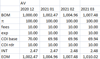
Right now, the cell with “2021 03” is a named range, CURRMO.
The numbers underneath it are sourced somewhere else in the workbook.
All of the stuff to the left of it is range-valued, hard-coded numbers.
Next month, first I will insert a column to the left of “2021 03”, copy-psv all of “2021 03” into the newly inserted column, then go update the Valuation Date which will feed into the far right column, thus making it “2021 04”.
Then, I go update all of the inputs that feed into the “2021 04” column. “2021 03” data is preserved.

What I want to do is set up a check that the new month’s BOM value is equal to last month’s EOM value.

The only way I can figure out how to do that right now is to use OFFSET. E.g., =OFFSET(CURRMO,1,0)-OFFSET(CURRMO,8,-1)

There must be a non-volatile way to do this such that this check will update to the new month’s values every month.

Certainly, I could INDEX on the column with CURRMO. However, I can’t figure out how to get the EOM value.

Well, this idea just popped into my head…tell me what you think:
Set the “2021 02” cell to PREVMO.
Keep “2021 03” as CURRMO.
For the monthly update, instead of inserting a column before CURRMO, insert it before PREVMO.
Then, copy-psv both the PREVMO and CURRMO columns one column to the left.
This should preserve the named ranges PREVMO & CURRMO as the last two columns, save their data in the appropriate columns, and then I can go update with this month’s data.

Now I can also set up an INDEX on the PREVMO column and it will always be the second-to-last column.

(Mind you I’d have to set up a named range for all of the data in each of those columns rather than just the header, but that’s neither here nor there. I can deal with that.)

Is there a better way? …or is that pretty good? “It’s not just good - it’s good enough!”

Do this.
Then, do:
3. Name a range for all of the data, call it “ALLDATA”, starting at column B (the one with “2020 12” in this example), through the current month.
4. HLOOKUP(PREVMO,ALLDATA,8,false)-HLOOKUP(CURRMO,ALLDATA,2,false)

You’re welcome.

1 Like

TYVM

There’s a lot of ways?
I think I would do…
index(BOM row, match(CURRMO, yearmonth row, 0))
and
index(EOM row, match(CURRMO, yearmonth row, 0) -1)

and also not add new named ranges. Just use cell references.

Also, if I’m trying to be a “good little actuary” I’d try to set it up so you don’t need to insert columns. The simplest version of that is to make the table go out to “2021 12” (or whatever) and leave it mostly empty. Then to put your calculated column to the left and just paste values every month.